

Diffusion coefficient of molecules using center of mass#
Kinisi includes the ability to calculate the mean-squared displacement and diffusion coefficient of the center of mass (or geometry) of molecules. This can be done for a single molecule or a collection of molecules. It is important to note that inclusion of rotational motion in the calculation of diffusion coeffiencents can lead to erronious results. This rotation can be eliminated from the calculation by taking the center of mass for each molecule.
[1]:
# This initialises the duecredit framework
%env DUECREDIT_ENABLE=yes
%env DUECREDIT_FILE=ase_COG.duecredit.p
import duecredit
duecredit.due.activate()

# Other imports for the notebook
import numpy as np
from ase.io import read
import matplotlib.pyplot as plt
from kinisi.analyze import DiffusionAnalyzer
import scipp as sc
env: DUECREDIT_ENABLE=yes
env: DUECREDIT_FILE=ase_COG.duecredit.p
We will use a simulation of ethene in ZSM-5 zeolite. This was run in DL_POLY, so we will use ASE to load in the trajectory (HISTORY) file.
[2]:
traj = read('ethene_zeo_HISTORY.gz', format='dlp-history', index=':')
We want to calculate the diffusion of the center of mass of the ethene molecule. This can be done by setting specie to None and specifying the indices of the molecules of interest in specie_indices as a scipp array. To define molecules, a scipp array should be passed under the specie_indices keyword with two dimensions atom and group_of_atoms.
The particle dimension should be the same size as the number of molecules, particle is the generic term in kinisi for a particle or group of particles.
The atoms in particle dimension should be the same size as the number of atoms in each each molecule.
In the example below we are calculating the msd and diffusion for 2 ethene molecules.
Only identical molecules are supported. The masses of the atoms in the molecules can be specified with masses. This must be a scipp array with the same length and dimension atoms in particle as a molecule.
[3]:
molecules = [[288, 289, 290, 291, 292, 293],
             [284, 295, 296, 297, 298, 299]]
mass    =  [12, 12, 1.008, 1.008, 1.008, 1.008]

params = {'specie': None,
           'time_step': 1.2e-03 * sc.Unit('ps'),
           'step_skip': 100 * sc.Unit('dimensionless'),
           'specie_indices': sc.array(dims=['particle', 'atoms in particle'],
                                      values=molecules,
                                      unit=sc.Unit('dimensionless')),
           'masses': sc.array(dims = ['atoms in particle'],
                              values = mass),
           'progress': False
           }
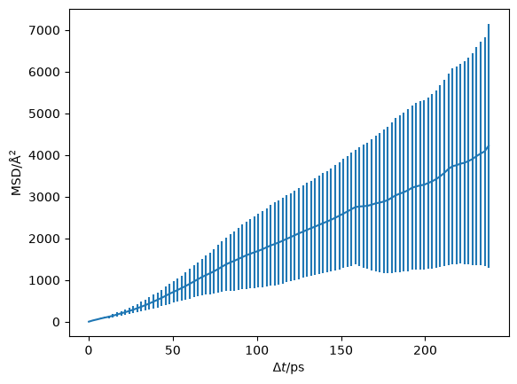
With the parameters set, we now calculate the mean squared-displacement.
[4]:
diff = DiffusionAnalyzer.from_ase(traj, **params)
[5]:
plt.errorbar(diff.dt.values[::20],
             diff.msd.values[::20],
             diff.msd.variances[::20]**0.5)
plt.ylabel('MSD/Å$^2$')
plt.xlabel(r'$\Delta t$/ps')
plt.show()
[6]:
start_of_diffusion = 60 * sc.Unit('ps')
diff.diffusion(start_of_diffusion, progress=False)
[7]:
diff.D
[7]:
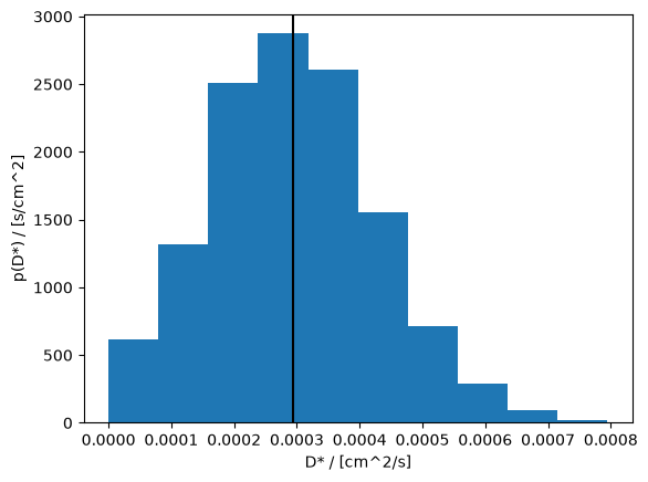
- (samples: 3200)float64cm^2/s0.00029+/-0.00013
Values:
array([0.00022129, 0.00046798, 0.00015388, ..., 0.00056652, 0.00022179,
       0.00025715], shape=(3200,))
[8]:
fig, ax = plt.subplots()

ax.hist(diff.D.values, density=True)
ax.axvline(sc.mean(diff.D).value, c='k')
ax.set_xlabel(f'D* / [{diff.D.unit}]')
ax.set_ylabel(f'p(D*) / [{(1 / diff.D.unit).unit}]')
plt.show()
[9]:
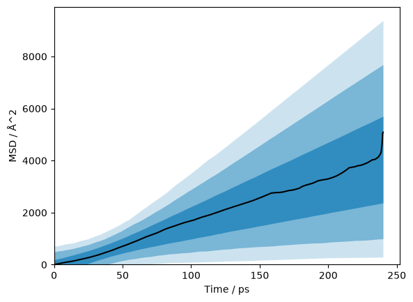
credible_intervals = [[16, 84], [2.5, 97.5], [0.15, 99.85]]
alpha = [0.6, 0.4, 0.2]

fig, ax = plt.subplots()
ax.plot(diff.dt.values, diff.msd.values, 'k-')
for i, ci in enumerate(credible_intervals):
    ax.fill_between(diff.dt.values,
                      *np.percentile(diff.distributions, ci, axis=1),
                      alpha=alpha[i],
                      color='#0173B2',
                      lw=0)
ax.set_xlabel(f'Time / {diff.dt.unit}')
ax.set_ylabel(f'MSD / {diff.msd.unit}')
ax.set_xlim(0, None)
ax.set_ylim(0, None)
plt.show()
The duecredit framework can then be used to output the relevant references that should be cited.
[10]:
from duecredit import due

due.dump()
DueCredit Report:
- kinisi: Bayesian analysis of mass transport from molecular dynamics simulations / kinisi (v 2.1.0) [1]
  - Atomic simulation environment which has been used for parsing. / kinisi.ase.ASEParser (v 2.1.0) [2]
  - Performs the Bayesian regression approach. / kinisi.diffusion.Diffusion.bayesian_regression (v 2.1.0) [3]
  - Implements the minimum eigenvalue method for matrix reconditioning. / kinisi.diffusion.minimum_eigenvalue_method (v 2.1.0) [4]
  - Uses the TOR scheme to find the unwrapped displacements of the atoms in the trajectory. / kinisi.parser.Parser.orthorhombic_calculate_displacements (v 2.1.0) [5]
  - Calculates the weighted molecular centre of mass using the pseudo-center of mass recentering method. / kinisi.pymatgen._calculate_centers_of_mass (v 2.1.0) [6]
- Scientific tools library / numpy (v 2.5.4) [7]

2 packages cited
5 modules cited
0 functions cited

References
----------

[1] McCluskey, A.R. et al., 2024. kinisi: Bayesian analysis of mass transport from molecular dynamics simulations. Journal of Open Source Software, 9(94), p.5984.
[2]
2026-10-29 09:37:07,742 [ERROR] Failed to process BibTeX file /tmp/tmp5kf2dsgi.bib: 'june'. (io.py:355)
ERRORED: 'june'
[3] McCluskey, A.R., Coles, S.W. & Morgan, B.J., 2024. Accurate Estimation of Diffusion Coefficients and their Uncertainties from Computer Simulation. Journal of Chemical Theory and Computation, 21(1), pp.79–87.
[4] Tabeart, J.M. et al., 2020. Improving the condition number of estimated covariance matrices. Tellus A: Dynamic Meteorology and Oceanography, 72(1), p.1696646.
[5] Bullerjahn, J.T. et al., 2023. Unwrapping NPT Simulations to Calculate Diffusion Coefficients. Journal of Chemical Theory and Computation, 19(11), pp.3406–3417.
[6] Richardson, H., Dunn, J. & McCluskey, A.R., 2025. On the estimation of center of mass in periodic systems. The Journal of Chemical Physics, 162(20).
[7] Van Der Walt, S., Colbert, S.C. & Varoquaux, G., 2011. The NumPy array: a structure for efficient numerical computation. Computing in Science & Engineering, 13(2), pp.22–30.