Diffusion coefficient from a VASP file

Previously, we looked at obtaining accurate estimates for the mean-squared displacement with kinisi. Here, we show that the same DiffusionAnalyzer can be used to evaluate the diffusion coefficient, using the kinisi methodology.

# This initialises the duecredit framework
%env DUECREDIT_ENABLE=yes
%env DUECREDIT_FILE=vasp_d.duecredit.p
import duecredit
duecredit.due.activate()

# Other imports for the notebook
import numpy as np
import matplotlib.pyplot as plt
import scipp as sc
from pymatgen.io.vasp import Xdatcar
from kinisi.analyze import DiffusionAnalyzer
rng = np.random.RandomState(42)

env: DUECREDIT_ENABLE=yes
env: DUECREDIT_FILE=vasp_d.duecredit.p

As with the previous example, params dictionary will describe the details about the simulation.

params = {'specie': 'Li',
          'time_step': 2.0 * sc.Unit('fs'),
          'step_skip': 50 * sc.Unit('dimensionless'),
          'progress': False
          }

In this example, we will add an additional key-value pair to the dictionary. This argument means that the diffusion coefficient will only be calculated in the xy plane of the simulation box.

params['dimension']= 'xy'

As with the previous example, we now use the from_xdatcar class method to construct the DiffusionAnalyzer object.

xd = Xdatcar('./example_XDATCAR.gz')
diff = DiffusionAnalyzer.from_xdatcar(xd, **params)

In the above cells, we parse and determine the uncertainty on the mean-squared displacement as a function of the timestep. We should visualise this, to check that we are observing diffusion in our material and to determine the timescale at which this diffusion begins.

fig, ax = plt.subplots()

ax.errorbar(diff.dt.values, diff.msd.values, np.sqrt(diff.msd.variances))
ax.set_xlabel(f'Time / {diff.dt.unit}')
ax.set_ylabel(f'MSD / {diff.msd.unit}')
ax.set_xlim(0, None)
ax.set_ylim(0, None)
plt.show()

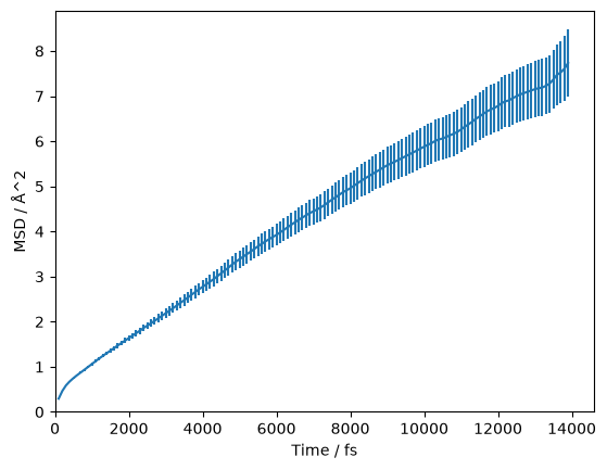
We can visualise this on a log-log scale, which helps to reveal the diffusive regime (the region where the gradient stops changing).

fig, ax = plt.subplots()

ax.errorbar(diff.dt.values, diff.msd.values, np.sqrt(diff.msd.variances))
ax.axvline(3000, color='g')
ax.set_xlabel(f'Time / {diff.dt.unit}')
ax.set_ylabel(f'MSD / {diff.msd.unit}')
ax.set_xscale('log')
ax.set_yscale('log')
plt.show()

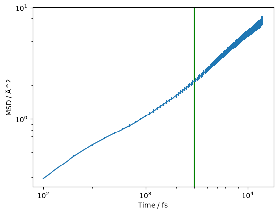
The green line at 3000 fs appears to be a reasonable estimate of the start of the diffusive regime. Therefore, we want to pass 3000 * sc.Units('fs') as the argument to the diffusion analysis below. At this stage, we pass the random_state argument to ensure reproducibility.

start_of_diffusion = 3000 * sc.Unit('fs')
diff.diffusion(start_of_diffusion, progress=False, random_state=rng)

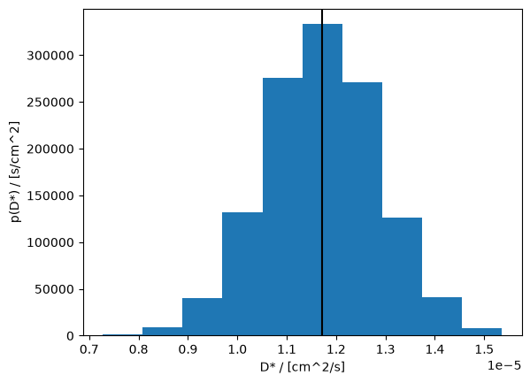
This method estimates the correlation matrix between the timesteps and uses posterior sampling to find the self-diffusion coefficient, \(D*\) and intercept. We can find the mean of the marginal posterior samples of \(D*\):

diff.D

kinisi.Samples

• • (samples: 3200)
    float64
    cm^2/s
    (1.17+/-0.12)e-05

    Values:
    array([1.18305711e-05, 1.19997173e-05, 1.27900411e-05, ...,
           1.18744657e-05, 9.91465543e-06, 1.22594724e-05], shape=(3200,))

The same for the intercept can be found from diff.intercept. A histogram of the marginal posterior probability distribution for \(D*\) can be plotted as shown below.

fig, ax = plt.subplots()

ax.hist(diff.D.values, density=True)
ax.axvline(sc.mean(diff.D).value, c='k')
ax.set_xlabel(f'D* / [{diff.D.unit}]')
ax.set_ylabel(f'p(D*) / [{(1 / diff.D.unit).unit}]')
plt.show()

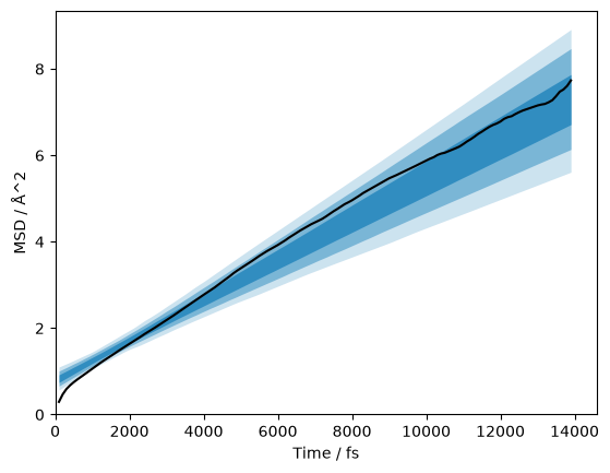
It is also possible to plot the posterior distribution of the models on the data. We represent this distribution with 1σ-, 2σ-, and 3σ-credible intervals. Here we remove the measured error bars, in the interest of clarity.

credible_intervals = [[16, 84], [2.5, 97.5], [0.15, 99.85]]
alpha = [0.6, 0.4, 0.2]

fig, ax = plt.subplots()
ax.plot(diff.dt.values, diff.msd.values, 'k-')
for i, ci in enumerate(credible_intervals):
    ax.fill_between(diff.dt.values,
                      *np.percentile(diff.distributions, ci, axis=1),
                      alpha=alpha[i],
                      color='#0173B2',
                      lw=0)
ax.set_xlabel(f'Time / {diff.dt.unit}')
ax.set_ylabel(f'MSD / {diff.msd.unit}')
ax.set_xlim(0, None)
ax.set_ylim(0, None)
plt.show()

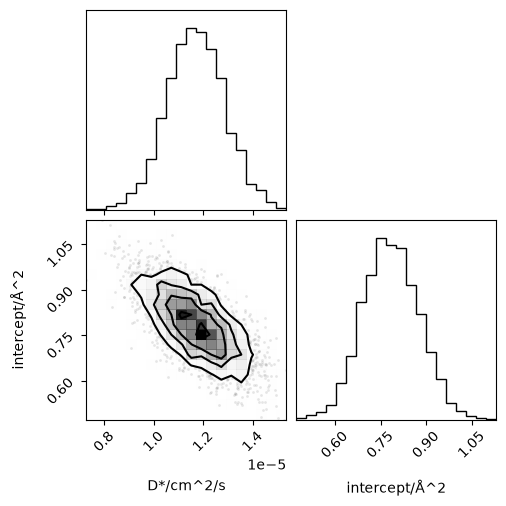
Finally, the joint posterior probability distribution for the diffusion coefficient and intercept can be visualised with the corner library.

from corner import corner

corner(np.array([i.values for i in diff.flatchain.values()]).T,
       labels=['/'.join([k, str(v.unit)]) for k, v in diff.flatchain.items()])
plt.show()

The duecredit framework can then be used to output the relevant references that should be cited.

from duecredit import due

due.dump()

DueCredit Report:
- kinisi: Bayesian analysis of mass transport from molecular dynamics simulations / kinisi (v 2.1.0) [1]
  - Performs the Bayesian regression approach. / kinisi.diffusion.Diffusion.bayesian_regression (v 2.1.0) [2]
  - Implements the minimum eigenvalue method for matrix reconditioning. / kinisi.diffusion.minimum_eigenvalue_method (v 2.1.0) [3]
  - Pymatgen, which as been used in parsing. / kinisi.pymatgen.PymatgenParser (v 2.1.0) [4]
- Scientific tools library / numpy (v 2.5.4) [5]

2 packages cited
3 modules cited
0 functions cited

References
----------

[1] McCluskey, A.R. et al., 2024. kinisi: Bayesian analysis of mass transport from molecular dynamics simulations. Journal of Open Source Software, 9(94), p.5984.
[2] McCluskey, A.R., Coles, S.W. & Morgan, B.J., 2024. Accurate Estimation of Diffusion Coefficients and their Uncertainties from Computer Simulation. Journal of Chemical Theory and Computation, 21(1), pp.79–87.
[3] Tabeart, J.M. et al., 2020. Improving the condition number of estimated covariance matrices. Tellus A: Dynamic Meteorology and Oceanography, 72(1), p.1696646.
[4] Ong, S.P. et al., 2013. Python Materials Genomics (pymatgen): A robust, open-source python library for materials analysis. Computational Materials Science, 68, pp.314–319.
[5] Van Der Walt, S., Colbert, S.C. & Varoquaux, G., 2011. The NumPy array: a structure for efficient numerical computation. Computing in Science & Engineering, 13(2), pp.22–30.