

Comparison with MDAnalysis#
MDAnalysis also contains a tool for calculating the mean-squared displacements. So why use kinisi over MDAnalysis?
Well, the approach taken by kinisi, which is outlined in the methodology, uses a high precision approach to estimate the diffusion coefficient and offers an accurate estimate of the variance in the mean-squared displacements and diffusion coefficient from a single simulation.
In this notebook, we will compare the results from MDAnalysis and kinisi. First we will import the kinisi.analyze.DiffusionAnalyzer and MDAnalysis.analysis.msd classes.
[1]:
# This initialises the duecredit framework
%env DUECREDIT_ENABLE=yes
%env DUECREDIT_FILE=mdanalysis.duecredit.p
import duecredit
duecredit.due.activate()

# Other imports for the notebook
import warnings

warnings.filterwarnings('ignore', category=DeprecationWarning)
warnings.filterwarnings('ignore', category=RuntimeWarning)
warnings.filterwarnings('ignore', category=UserWarning)

import numpy as np
import scipp as sc

import kinisi
from kinisi.analyze import DiffusionAnalyzer
import MDAnalysis.analysis.msd as msd
from MDAnalysis.transformations.nojump import NoJump
env: DUECREDIT_ENABLE=yes
env: DUECREDIT_FILE=mdanalysis.duecredit.p
/opt/hostedtoolcache/Python/3.12.15/x64/lib/python3.12/site-packages/duecredit/injections/injector.py:340: TqdmWarning: IProgress not found. Please update jupyter and ipywidgets. See https://ipywidgets.readthedocs.io/en/stable/user_install.html
  mod = self._orig_import(name, *args, **kwargs)
Next, we are going to need to do a little ‘magic’ to get MDAnalysis to read an extended xyz file. Luckily ASE can help us out.
[2]:
from ase.io import read
from MDAnalysis import Universe
import os
Since this trajectory has a triclinic cell; we need to extract the cell dimensions and pass them to MDAnalysis.
[3]:
# The file we want to load is in the test cases for kinisi,
# so will need to get the path to it.
path_to_file = os.path.join(os.path.dirname(kinisi.__file__),
                            'tests/inputs/LiPS.exyz')
atoms = read(path_to_file, format='extxyz', index=':')

cell_dimensions = []
for frame in atoms:
    lengths = frame.cell.lengths()
    angles = frame.cell.angles()
    cell = [*lengths, *angles]
    cell_dimensions.append(cell)
We now have the cell dimensions (\(a, b, c, \alpha, \beta, \gamma\)) in an array. We now need to create an MDAnalysis universe and apply these dimension to it.
[4]:
u = Universe(path_to_file,
             path_to_file,
             format='XYZ',
             topology_format='XYZ',
             dt=20.0/1000)
for ts, dims in zip(u.trajectory, cell_dimensions):
    ts.dimensions = dims
Now we add an unwrapping transformation to the universe, create the MSD object, run the analysis, and extract the results as a timeseries.
[5]:
u.trajectory.add_transformations(NoJump())
MSD = msd.EinsteinMSD(u,
                      select='type LI',
                      msd_type='xyz',
                      fft=True,
                      verbose=False)
MSD.run(verbose=False)

mda_MSD = MSD.results.timeseries
mda_dt = MSD.results.delta_t_values
With the result from MDAnalysis in one hand we can now do the same thing in kinisi with the other. Here, we use the custom dt functionality that is available in kinisi, with this we pass a scipp array of time intervals to compute the MSD over. Note, that the custom dt must be represented within possible simulation time intervals, or an error will be raised.
[6]:
params = {'specie': 'LI',
          'time_step': 0.001 * sc.Unit('ps'),
          'step_skip': 20 * sc.units.dimensionless,
          'progress': False,
          'dt': sc.arange(dim='time interval', start=0.1 * sc.Unit('ps'),
                         stop=4.0 * sc.Unit('ps'),
                         step=0.1 * sc.Unit('ps'))
          }

kinisi_from_universe = DiffusionAnalyzer.from_universe(u, **params)
kinisi_MSD = kinisi_from_universe.msd
time = kinisi_from_universe.dt
Putting the two analyses’ together, we can plot for comparison.
[7]:
import matplotlib.pyplot as plt

plt.plot(time, kinisi_MSD, label='Kinisi MSD', c='#ff7f0e')
plt.plot(mda_dt, mda_MSD, label='MDanalysis', ls='--')
plt.ylabel('MSD (Å$^2$)')
plt.xlabel('Diffusion time (ps)')
plt.legend()


plt.show()
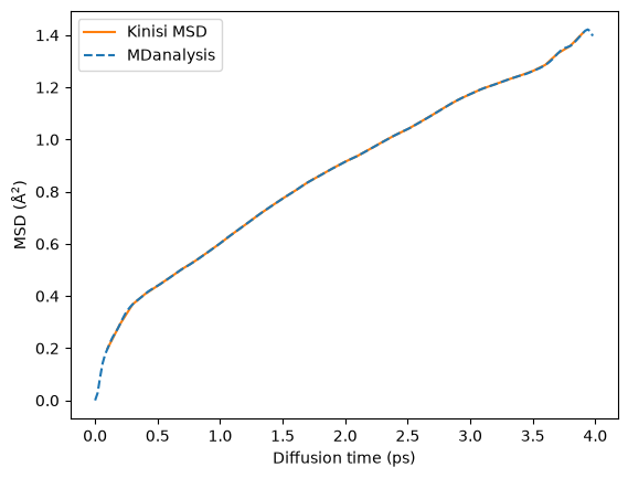
The results overlap almost entirely.
We can now extract an accurate estimation of the variance in the observed MSD from kinisi. For clarity, we will use array indexing to remove every other data point.
[8]:
plt.errorbar(kinisi_from_universe.dt.values,
             kinisi_from_universe.msd.values,
             np.sqrt(kinisi_from_universe.msd.variances),
             c='#ff7f0e')
plt.ylabel(r'MSD/Å$^2$')
plt.xlabel(r'$\Delta t$/ps')
plt.show()
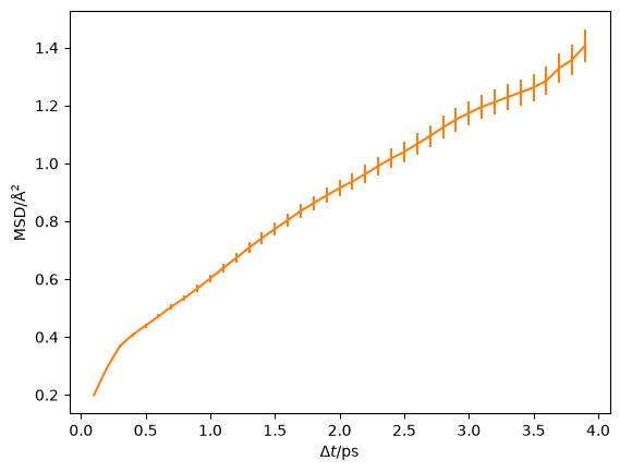
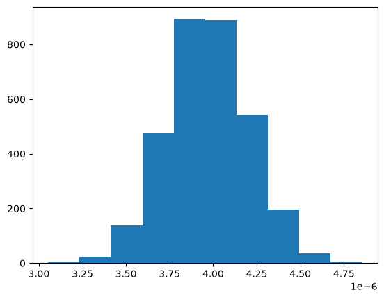
We can also calculate estimated diffusion coefficient, and the associated uncertainty, with kinisi.
[9]:
kinisi_from_universe.diffusion(1.5 * sc.Unit('ps'))
kinisi_from_universe.D
Likelihood Sampling: 100%|██████████| 1500/1500 [00:00<00:00, 2725.39it/s]
[9]:
- (samples: 3200)float64cm^2/s(3.97+/-0.23)e-06
Values:
array([4.60137827e-06, 3.45742025e-06, 3.79842305e-06, ...,
       4.32902631e-06, 3.89597364e-06, 3.84914395e-06], shape=(3200,))
[10]:
plt.hist(kinisi_from_universe.D.values)
[10]:
(array([  4.,  23., 139., 474., 893., 889., 542., 195.,  37.,   4.]),
 array([3.05326562e-06, 3.23327469e-06, 3.41328376e-06, 3.59329283e-06,
        3.77330190e-06, 3.95331097e-06, 4.13332004e-06, 4.31332911e-06,
        4.49333818e-06, 4.67334725e-06, 4.85335632e-06]),
 <BarContainer object of 10 artists>)
[11]:
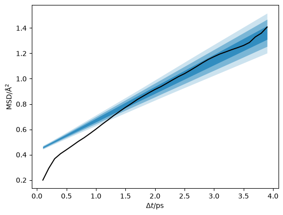
credible_intervals = [[16, 84], [2.5, 97.5], [0.15, 99.85]]
alpha = [0.6, 0.4, 0.2]

plt.plot(kinisi_from_universe.dt, kinisi_from_universe.msd, 'k-')
for i, ci in enumerate(credible_intervals):
    plt.fill_between(kinisi_from_universe.dt.values,
                     *np.percentile(kinisi_from_universe.distributions,
                                    ci,
                                    axis=1),
                     alpha=alpha[i],
                     color='#0173B2',
                     lw=0)
plt.ylabel('MSD/Å$^2$')
plt.xlabel(r'$\Delta t$/ps')
plt.show()
The duecredit framework can then be used to output the relevant references that should be cited.
[12]:
from duecredit import due

due.dump()
DueCredit Report:
- Molecular simulation analysis library / MDAnalysis (v 2.11.0) [1, 2]
  - FCA fast correlation algorithm, Mean Squared Displacements with tidynamics / MDAnalysis.analysis.msd (v 2.11.0) [3, 4]
  - QCProt implementation / MDAnalysis.lib.qcprot (v 2.11.0) [5, 6]
  - Works through the orthogonal case for unwrapping, and proposes the non-orthogonal approach. / MDAnalysis.transformations.nojump (v 2.11.0) [7]
- kinisi: Bayesian analysis of mass transport from molecular dynamics simulations / kinisi (v 2.1.0) [8]
  - Performs the Bayesian regression approach. / kinisi.diffusion.Diffusion.bayesian_regression (v 2.1.0) [9]
  - Implements the minimum eigenvalue method for matrix reconditioning. / kinisi.diffusion.minimum_eigenvalue_method (v 2.1.0) [10]
- Scientific tools library / numpy (v 2.5.4) [11]

3 packages cited
5 modules cited
0 functions cited

References
----------

[1] Gowers, R. et al., 2016. MDAnalysis: A Python Package for the Rapid Analysis of Molecular Dynamics Simulations. In Proceedings of the 15th Python in Science Conference. SciPy.  SciPy, pp. 98–105.
[2] Michaud‐Agrawal, N. et al., 2011. MDAnalysis: A toolkit for the analysis of molecular dynamics simulations. Journal of Computational Chemistry, 32(10), pp.2319–2327.
[3] de Buyl, P., 2018. tidynamics: A tiny package to compute the dynamics of stochastic and molecular simulations. Journal of Open Source Software, 3(28), p.877.
[4] Calandrini, V. et al., 2011. nMoldyn - Interfacing spectroscopic experiments, molecular dynamics simulations and models for time correlation functions. École thématique de la Société Française de la Neutronique, 12, pp.201–232.
[5]
2026-10-29 09:37:32,623 [ERROR] Failed to process BibTeX file /tmp/tmpj7uezp0q.bib: 'june'. (io.py:355)
ERRORED: 'june'
[6] Liu, P., Agrafiotis, D.K. & Theobald, D.L., Fast determination of the optimal rotational matrix for macromolecular superpositions. Journal of Computational Chemistry, 31(7), pp.1561–1563.
[7]
2026-10-29 09:37:32,933 [ERROR] Failed to process BibTeX file /tmp/tmp540_dapy.bib: 'sept'. (io.py:355)
ERRORED: 'sept'
[8] McCluskey, A.R. et al., 2024. kinisi: Bayesian analysis of mass transport from molecular dynamics simulations. Journal of Open Source Software, 9(94), p.5984.
[9] McCluskey, A.R., Coles, S.W. & Morgan, B.J., 2024. Accurate Estimation of Diffusion Coefficients and their Uncertainties from Computer Simulation. Journal of Chemical Theory and Computation, 21(1), pp.79–87.
[10] Tabeart, J.M. et al., 2020. Improving the condition number of estimated covariance matrices. Tellus A: Dynamic Meteorology and Oceanography, 72(1), p.1696646.
[11] Van Der Walt, S., Colbert, S.C. & Varoquaux, G., 2011. The NumPy array: a structure for efficient numerical computation. Computing in Science & Engineering, 13(2), pp.22–30.