Jump diffusion coefficient from a VASP file

Previously, we looked at obtaining accurate estimates for the self-diffusion coefficient with kinisi. Here, we look at how we can use kinisi to compute the jump diffusion coefficient.

# This initialises the duecredit framework
%env DUECREDIT_ENABLE=yes
%env DUECREDIT_FILE=vasp_dj.duecredit.p
import duecredit
duecredit.due.activate()

# Other imports for the notebook
import numpy as np
import matplotlib.pyplot as plt
import scipp as sc
from kinisi.analyze import JumpDiffusionAnalyzer
from pymatgen.io.vasp import Xdatcar
np.random.seed(42)
rng = np.random.RandomState(42)

env: DUECREDIT_ENABLE=yes
env: DUECREDIT_FILE=vasp_dj.duecredit.p

As with the previous example, params dictionary will describe the details about the simulation.

params = {'specie': 'Li',
          'time_step': 2.0 * sc.Unit('fs'),
          'step_skip': 50 * sc.Unit('dimensionless'),
          'progress': False
          }

Again, we will add an additional key-value pair to the dictionary. This time, it is the “number of system particles”.

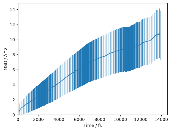
The computation of the jump diffusion coefficient requires the mean-squared total displacement (MSTD) to be found. The MSTD is the displacement of the centre of mass of all selected particles (the specie) in the simulation. This means that for a given simulation, there is only a single “atom” or system particle observed. Just a single system particle means that the statistics for the jump diffusion coefficient can be quite poor.

We can improve the statistics in the computation of the jump diffusion coefficient by splitting the simulation up into some number of individual simulations (in space) and therefore system particles. Then the MSTD over each of these system particles can be found, leading to reduced noise in the uncertainty estimation. The system_particles parameter defined how many times the simulation should be split, here we use 32 system particles.

params['system_particles']= 32

xd = Xdatcar('./example_XDATCAR.gz')
diff = JumpDiffusionAnalyzer.from_xdatcar(xd, **params)

In the above cells, we parse and determine the uncertainty on the mean-squared displacement as a function of the timestep. We should visualise this, to check that we are observing diffusion in our material and to determine the timescale at which this diffusion begins.

fig, ax = plt.subplots()

ax.errorbar(diff.dt.values, diff.mstd.values, np.sqrt(diff.mstd.values))
ax.set_xlabel(f'Time / {diff.dt.unit}')
ax.set_ylabel(f'MSD / {diff.mstd.unit}')
ax.set_xlim(0, None)
ax.set_ylim(0, None)
plt.show()

We compare the variance with when there are fewer system particles used below. Note, the logarithmic y-axis.

params['system_particles']= 4
diff_fewer = JumpDiffusionAnalyzer.from_xdatcar(xd, **params)

fig, ax = plt.subplots()

ax.plot(diff.dt.values, diff.mstd.variances, label='16 system particles')
ax.plot(diff_fewer.dt.values, diff_fewer.mstd.variances, label='8 system particles')
ax.set_xlabel(f'Time / {diff.dt.unit}')
ax.set_ylabel(f'MSTD variance / {(1 * diff.mstd.unit ** 2).unit}')
ax.set_xlim(0, None)
# ax.set_ylim(0, None)
ax.set_yscale('log')
ax.legend()

<matplotlib.legend.Legend at 0x7d84a00d6600>

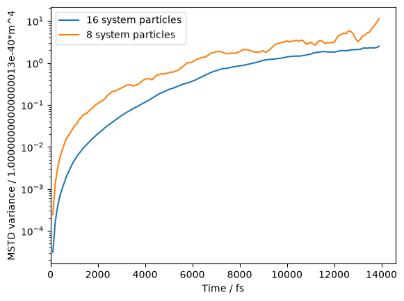
This same process is relevant to the computation of the conductivity analyser, as the mean-squared charge distribution (MSCD) is the displacement of charge in the system and, therefore, suffers similarly as there is only a single “system particle” in the simulation.

We can visualise the data with 16 system particles on a log-log scale, which helps to reveal the diffusive regime (the region where the gradient stops changing).

fix, ax = plt.subplots()

ax.errorbar(diff.dt.values, diff.mstd.values, np.sqrt(diff.mstd.values))
ax.axvline(4000, color='g')
ax.set_xlabel(f'Time / {diff.dt.unit}')
ax.set_ylabel(f'MSTD / {diff.mstd.unit}')
ax.set_yscale('log')
ax.set_xscale('log')
plt.show()

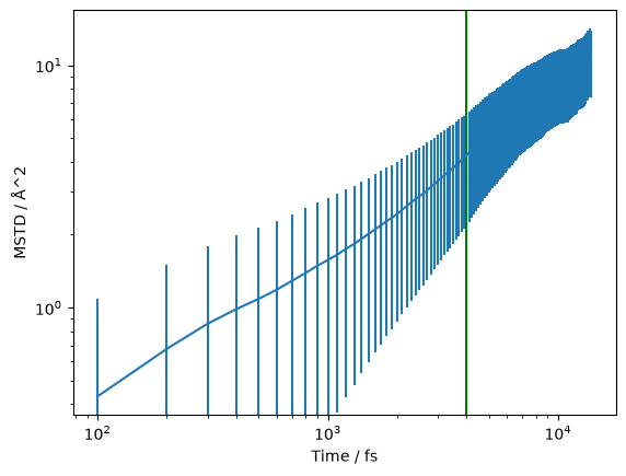
The green line at 4000 fs appears to be a reasonable estimate of the start of the diffusive regime. Therefore, we want to pass 4000 * sc.Units('fs') as the argument to the diffusion analysis below. At this stage, we pass the random_state argument to ensure reproducibility.

start_of_diffusion = 4000 * sc.Unit('fs')
diff.jump_diffusion(start_of_diffusion, progress=False, random_state=rng)

/opt/hostedtoolcache/Python/3.12.15/x64/lib/python3.12/site-packages/duecredit/collector.py:439: UserWarning: The generalised least squares gradient differs from the ordinary least squares estimate by 3.8 times the spread expected from the noise in the data (z = -3.82). A difference this large indicates that the covariance matrix may be unreliable, or that a straight line does not describe the data from start_dt onwards, and that the diffusion coefficient may be wrong. Consider a later start_dt, refitting with recondition=True, or inspecting the eigenvalues of Diffusion.covariance_matrix.
  return func(*fargs, **fkwargs)

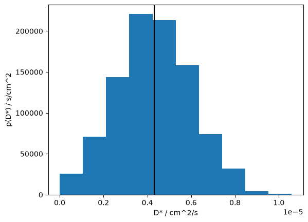
This method estimates the correlation matrix between the timesteps and uses posterior sampling to find the jump diffusion coefficient, \(D*\) and intercept. We can find the mean of the marginal posterior samples of \(D*\):

diff.D_J

kinisi.Samples

• • (samples: 3200)
    float64
    cm^2/s
    (4.3+/-1.7)e-06

    Values:
    array([4.81431236e-06, 3.76545676e-06, 5.30195190e-06, ...,
           6.57978731e-06, 5.21636874e-06, 6.31992397e-06], shape=(3200,))

Or we can get all of the sampled values from one of these objects.

diff.D_J.values

array([4.81431236e-06, 3.76545676e-06, 5.30195190e-06, ...,
       6.57978731e-06, 5.21636874e-06, 6.31992397e-06], shape=(3200,))

The same for the intercept can be found for diff.intercept. A histogram of the marginal posterior probability distribution for \(D*\) can be plotted as shown below.

fig, ax = plt.subplots()

ax.hist(diff.D_J.values, density=True)
ax.axvline(sc.mean(diff.D_J).value, c='k')
ax.set_xlabel(f'D* / {diff.D_J.unit}')
ax.set_ylabel(f'p(D*) / {(1 / diff.D_J.unit).unit}')
plt.show()

Having completed the analysis, we can save the object for use later (such as downstream by a plotting script).

diff.to_hdf5('example.hdf')

The data is saved in a HDF5 file format which helps us efficiently store our data. We can then load the data with the following class method.

loaded_diff = JumpDiffusionAnalyzer.from_hdf5('example.hdf')

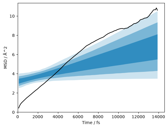
We can plot the data with the credible intervals from the \(D\) and \(D_{\text{offset}}\) distribution.

credible_intervals = [[16, 84], [2.5, 97.5], [0.15, 99.85]]
alpha = [0.6, 0.4, 0.2]

fig, ax = plt.subplots()
ax.plot(loaded_diff.dt.values, loaded_diff.mstd.values, 'k-')
for i, ci in enumerate(credible_intervals):
    ax.fill_between(loaded_diff.dt.values,
                     *np.percentile(loaded_diff.distributions, ci, axis=1),
                     alpha=alpha[i],
                     color='#0173B2',
                     lw=0)
ax.set_xlabel(f'Time / {diff.dt.unit}')
ax.set_ylabel(f'MSD / {diff.mstd.unit}')
ax.set_xlim(0, None)
ax.set_ylim(0, None)
plt.show()

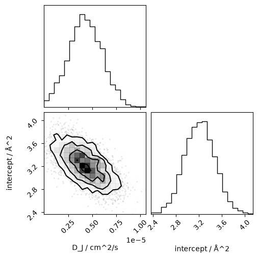
We can then do things like plot the joint probability distribution for the diffusion coefficient and intercept.

from corner import corner

corner(np.array([i.values for i in loaded_diff.flatchain.values()]).T,
       labels=[' / '.join([k, str(v.unit)])
               for k, v in loaded_diff.flatchain.items()])
plt.show()

The duecredit framework can then be used to output the relevant references that should be cited.

from duecredit import due

due.dump()

DueCredit Report:
- kinisi: Bayesian analysis of mass transport from molecular dynamics simulations / kinisi (v 2.1.0) [1]
  - Performs the Bayesian regression approach. / kinisi.diffusion.Diffusion.bayesian_regression (v 2.1.0) [2]
  - Implements the minimum eigenvalue method for matrix reconditioning. / kinisi.diffusion.minimum_eigenvalue_method (v 2.1.0) [3]
  - Pymatgen, which as been used in parsing. / kinisi.pymatgen.PymatgenParser (v 2.1.0) [4]
- Scientific tools library / numpy (v 2.5.4) [5]

2 packages cited
3 modules cited
0 functions cited

References
----------

[1] McCluskey, A.R. et al., 2024. kinisi: Bayesian analysis of mass transport from molecular dynamics simulations. Journal of Open Source Software, 9(94), p.5984.
[2] McCluskey, A.R., Coles, S.W. & Morgan, B.J., 2024. Accurate Estimation of Diffusion Coefficients and their Uncertainties from Computer Simulation. Journal of Chemical Theory and Computation, 21(1), pp.79–87.
[3] Tabeart, J.M. et al., 2020. Improving the condition number of estimated covariance matrices. Tellus A: Dynamic Meteorology and Oceanography, 72(1), p.1696646.
[4] Ong, S.P. et al., 2013. Python Materials Genomics (pymatgen): A robust, open-source python library for materials analysis. Computational Materials Science, 68, pp.314–319.
[5] Van Der Walt, S., Colbert, S.C. & Varoquaux, G., 2011. The NumPy array: a structure for efficient numerical computation. Computing in Science & Engineering, 13(2), pp.22–30.